Flow Solver Tutorials
Please note that in addition to the tutorials contained here, there are a number of additional resources available in the Training Workshops area of the site. Video footage from approximately 15 in-depth training sessions over a 2-day period are available for viewing. These sessions covered all of the major application areas of FUN3D at the time they were produced.
Flow Solver Tutorial #1
Inviscid flow solve
Intent: Demonstrate simple inviscid execution of the baseline flow solver
This tutorial will describe how to set up and obtain a coarse-grid inviscid flow solution with FUN3D v13.3.
All the grid and input files may be downloaded as described below. Note that the grid for this case is very coarse and is intended for demonstration, rather than accurate aerodynamic analysis. The geometry consists of a stand-alone ONERA M6 (OM6) wing with a symmetry boundary condition imposed at the wing root.
The reader should be familiar with the flow solver inputs (See FUN3D Manual: Appendix B FUN3D Input Files).
Compilation and linking
(See FUN3D Manual: Appendix A Installation).
Files
Download (0.2MB) and gunzip/untar the files:$ tar zvxf flow_demo1.tar.gz x flow_demo1/ x flow_demo1/fun3d.nml x flow_demo1/om6inviscid.fgrid x flow_demo1/om6inviscid.mapbc
The namelist file, fun3d.nml, is used to control the execution
of the solver (initial conditions, physical models, etc.).
The following is a very simple example for basic execution.
There are more aggressive strategies available,
but this will be sufficient to get started.
This example namelist file relies on defaults and only modifies values relevant to this case.
 &project
    project_rootname = "om6inviscid"
    case_title = "OM6 Simple Inviscid Flow Solve Tutorial"
 /

 &governing_equations
    viscous_terms = "inviscid"
 /

 &reference_physical_properties
    mach_number     = 0.7
    angle_of_attack = 2.0
 /

 &force_moment_integ_properties
    area_reference =    1.067634
    x_moment_length =   0.673700
    y_moment_length =   1.020000
    x_moment_center =   0.168425
 /

 &nonlinear_solver_parameters
    schedule_cfl =  10.0  200.0
 /

 &code_run_control
    steps              = 1000
    stopping_tolerance = 1.0E-15
    restart_write_freq = 1000
    restart_read = "off"
 /

 &raw_grid
   grid_format = "fast"
   data_format = "ascii"
   patch_lumping = "none"
 /
Although not necessary,
we will assume that the flow solver executable (nodet or nodet_mpi)
has been installed in your search path to simplify the discussion to follow.
Therefore, we will not reference an explicit path to the executable,
but instead simply invoke directly like any other installed software.
Execute the flow solver
For sequential, i.e., single-processor, execution
the flow solver is invoked as follows,
where the --animation_freq -1 command line option
is specified to provide Tecplot visualization output
for the solid boundary surfaces:
% nodet --animation_freq -1
FUN3D 12.2-63280 started 12/20/2010 at 15:40:12.695 with 1 MPI processes
Contents of file fun3d.nml below------------------------------------------------
  &project
     project_rootname = "om6inviscid"

[...]

 Done.
For parallel (multiple-processor) execution,
the flow solver is invoked through an MPI
command like mpirun, aprun, or mpiexec depending
on your local environment.
It is assumed that your system is configured
for some implementation of MPI
and that all processors have access to the case directory
and to the nodet_mpi executable.
For an OpenMPI-based environment, the run command may look like the following:
% mpirun -machinefile your.machines -np 8 nodet_mpi --animation_freq -1
FUN3D 12.2-63280 started 12/20/2010 at 15:40:12.695 with 8 MPI processes
Contents of file fun3d.nml below------------------------------------------------
  &project
     project_rootname = "om6inviscid"

[...]

 Done.
Post-process the results
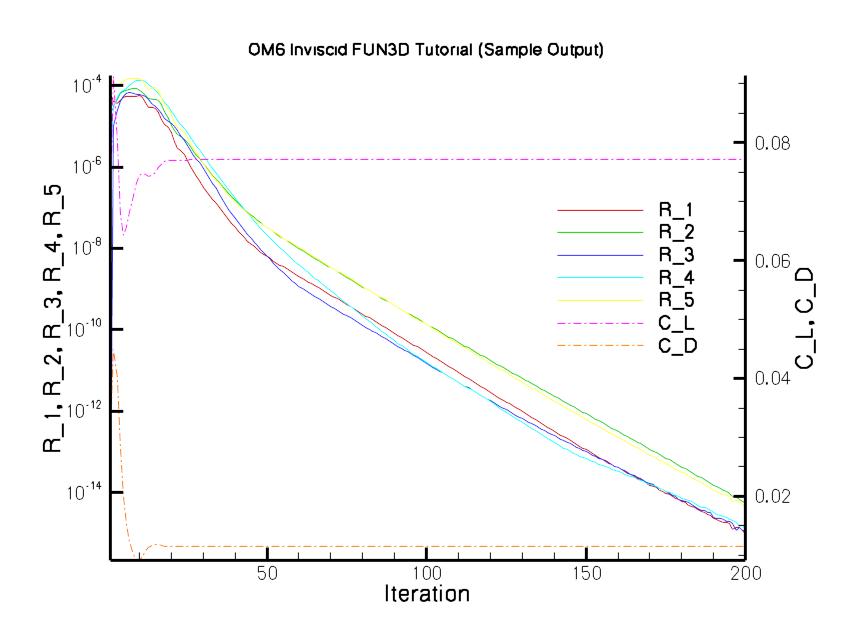
The figure below is a representative convergence history for this case.
The residual information is available in the file om6inviscid_hist.dat
and is in the Tecplot format.
The residual values (R_1, R_2, R_3, R_4, R_5)
represent the convergence of the 5 equations of state
(mass, x-momentum, y-momentum, z-momentum, and energy, respectively).
They are plotted using a Log scale below.
The Tecplot surface visualization file om6inviscid_tec_boundary.dat
is the result of the --animation_freq -1 command line option.
This file contains the primitive variables on each solid boundary surface.
Note: This file may have a .plt or .szplt suffix if your FUN3D is configured
to use the binary Tecplot I/O libraries.
Flow Solver Tutorial #2
Turbulent flow solve
Intent: Demonstrate simple turbulent execution of the baseline flow solver
This tutorial will describe how to set up and obtain a coarse-grid turbulent flow solution with FUN3D v13.3.
All the grid and input files may be downloaded as described below. Note that the grid for this case is very coarse and is intended for demonstration rather than accurate aerodynamic analysis. The geometry consists of a stand-alone ONERA M6 (OM6) wing with a symmetry boundary condition imposed at the wing root.
The reader should be familiar with the flow solver inputs (See FUN3D Manual: Appendix B FUN3D Input Files).
Compilation and linking
(See FUN3D Manual: Appendix A Installation).
Files
Download (1.4MB) and gunzip/untar the files:$ tar zvxf flow_demo2.tar.gz x flow_demo2/ x flow_demo2/fun3d.nml-initial x flow_demo2/fun3d.nml-restart x flow_demo2/om6viscous_symmetry.fgrid x flow_demo2/om6viscous_symmetry.mapbcAs for the first flow solver tutorial, a namelist file,
fun3d.nml, is used to control the execution of the solver
(initial conditions, physical models, etc.).
In this tutorial, we will run the code twice: once to initialize
the flow and a second time to converge the solution to machine precision.
For the first phase,
cp fun3d-nml-initial fun3d.nmlwhich sets up a bare bones example for basic execution:
 &project
    project_rootname = "om6viscous_symmetry"
    case_title = "OM6 Simple Turbulent Flow Solve Tutorial"
 /

 &reference_physical_properties
    temperature_units = "Rankine"
    mach_number     = 0.7
    reynolds_number = 3000000.0
    temperature     = 460.0
    angle_of_attack = 2.0
 /

 &force_moment_integ_properties
    area_reference  = 1.067634
    x_moment_length = 0.673700
    y_moment_length = 1.020000
    x_moment_center = 0.168425
 /

 &nonlinear_solver_parameters
    schedule_cfl     =  10.0   200.0
    schedule_cflturb =   1.0    20.0
 /

 &code_run_control
    steps              = 1000
    stopping_tolerance = 1.0E-15
    restart_write_freq = 1000
    restart_read = "off"
 /

 &raw_grid
  grid_format = "fast"
  data_format = "ascii"
  patch_lumping = "none"
 /
Although not necessary,
we will assume that the flow solver executable (nodet or nodet_mpi)
has been installed in your search path to simplify the discussion to follow.
Therefore, we will not reference an explicit path to the executable,
but instead simply invoke directly like any other installed software.
Execute the flow solver
For sequential, i.e., single-processor, execution
the flow solver is invoked as follows,
where the --animation_freq -1 command line option
is specified to provide Tecplot visualization output
for the solid boundary surfaces:
% nodet --animation_freq -1
FUN3D 12.2-63280 started 12/20/2010 at 15:40:12.695 with 1 MPI processes
Contents of file fun3d.nml below------------------------------------------------
  &project
     project_rootname = "om6viscous_symmetry"

[...]

 Done.
For parallel (multiple-processor) execution,
the flow solver is invoked through an MPI
command like mpirun, aprun, or mpiexec depending
on your local environment.
It is assumed that your system is configured
for some implementation of MPI
and that all processors have access to the case directory
and to the nodet_mpi executable.
For an OpenMPI-based environment, the run command may look like the following:
% mpirun -machinefile your.machines -np 8 nodet_mpi --animation_freq -1
FUN3D 12.2-63280 started 12/20/2010 at 15:40:12.695 with 8 MPI processes
Contents of file fun3d.nml below------------------------------------------------
  &project
     project_rootname = "om6viscous_symmetry"

[...]

 Done.
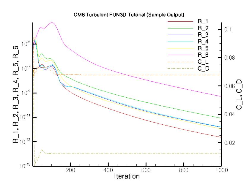
The resulting convergence history is shown in the following plot.
While overall convergence is good, we will restart the solution to continue to converge the solution to machine precision. For this we will need to modify the FUN3D namelist input filefun3d.nml.
The modifications include:
(1) Changing the CFL schedules (nonlinear_solver_parameters namelist
variables schedule_cfl and schedule_cflturb)
since the values were ramped to their maximum values during the initial run;
and
(2) Restarting the solution
(code_run_control namelist variable restart_read).
Note that the restart will run another 1,000 steps
unless the density residual falls below the given threshold (1.0e-15).
The tarball contains this modified fun3d.nml file; so
cp fun3d.nml-restart fun3d.nmlwhich should contain the following:
 &project
    project_rootname = "om6viscous_symmetry"
    case_title = "OM6 Simple Turbulent Flow Solve Tutorial"
 /

 &reference_physical_properties
    angle_of_attack   = 2.0
    mach_number       = 0.7
    reynolds_number   = 3000000.0
    temperature       = 460.0
    temperature_units = "Rankine"
 /

 &force_moment_integ_properties
    area_reference =  1.067634
    x_moment_length = 0.673700
    y_moment_length = 1.020000
    x_moment_center = 0.168425
 /

 &nonlinear_solver_parameters
    schedule_cfl     = 200.0  200.0
    schedule_cflturb =  20.0   20.0
 /

 &code_run_control
    steps              = 1000
    stopping_tolerance = 1.0E-15
    restart_write_freq = 1000
    restart_read = "on"
 /

 &raw_grid
  grid_format = "fast"
  data_format = "ascii"
  patch_lumping = "none"
 /
Execution of the flow solver using the above FUN3D namelist is
conducted in the same manner as for the initial invocation.
For example, parallel execution is invoked through mpirun as before.
% mpirun -machinefile your.machines -np 8 nodet_mpi --animation_freq -1
FUN3D 12.2-63280 started 12/20/2010 at 15:40:12.695 with 8 MPI processes
Contents of file fun3d.nml below------------------------------------------------
  &project
     project_rootname = "om6viscous_symmetry"

[...]

 Done.
Post-process the results
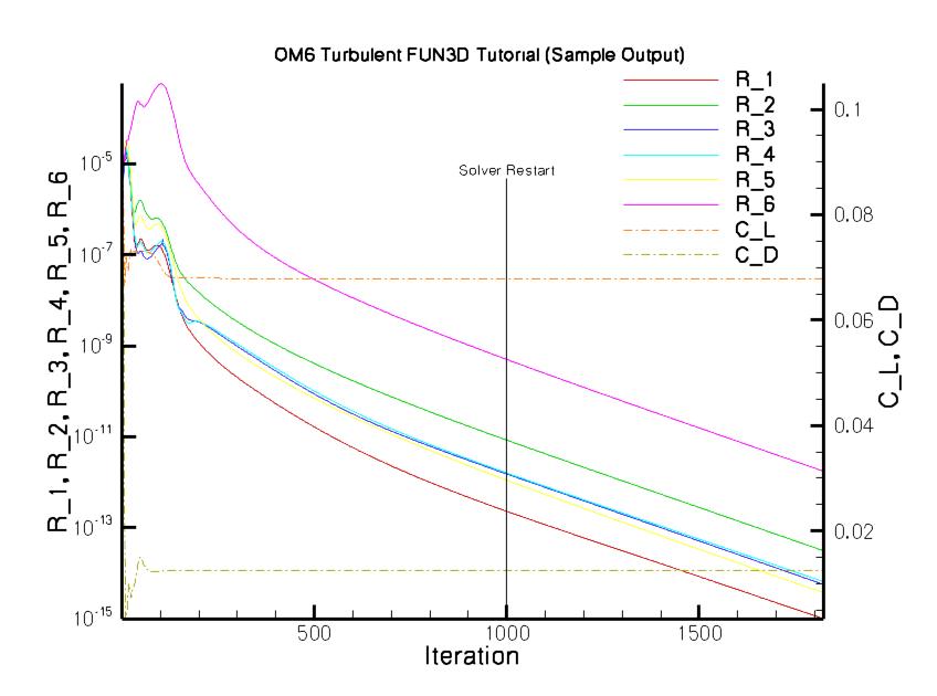
The following is a representative convergence history for this case.
The residual information is available in the file om6viscous_symmetry_hist.dat
and is in the Tecplot format.
The residual values (R_1, R_2, R_3, R_4, R_5, R_6) represent
the convergence of the 5 equations of state
(mass, x-momentum, y-momentum, z-momentum, energy,
and the 1 Eqn. SA model respectively).
They are plotted using a Log scale below.
The result of the above execution will also generate
the Tecplot file om6viscous_symmetry_tec_boundary.dat
for examination of solid surface quantities.
Flow Solver Tutorial #3
Merge VGRID mesh into mixed elements and run solution
Intent: Demonstrate how to merge tetrahedral VGRID mesh into mixed elements and run turbulent flow solution
This tutorial will describe how to merge a tetrahedral VGRID mesh into mixed elements and execute a turbulent flow solve using FUN3D v13.3.
The grid and input files for this example are from the AIAA DPW-2 workshop and can be downloaded as described below. Note that the grids for this case are very coarse and are intended for demonstration rather than accurate aerodynamic analysis. The geometry consists of a wing-body configuration with half-plane symmetry.
The reader should be familiar with the flow solver inputs (See FUN3D Manual: Appendix B FUN3D Input Files).
Compilation and linking
(See FUN3D Manual: Appendix A Installation).
Files
Download (68MB) and gunzip/untar:$ tar zvxf flow_demo3.tar.gz x flow_demo3/ x flow_demo3/f6wbnc.bc x flow_demo3/f6wbnc.cogsg x flow_demo3/f6wbnc.mapbc x flow_demo3/f6wbnc.poin1 x flow_demo3/fun3d.nml
Note that you need the .poin1 file for merging the grid—normally
this file is not required to process the raw tetrahedral grid.
As with previous flow solver tutorials,
a fun3d.nml namelist file is used to control the execution of the solver
(initial conditions, physical models, etc.).
The following is a very simple example for illustrative purposes;
more advanced strategies are available but not covered here.
 &project
    project_rootname = "f6wbnc.merged"
    case_title = "Merged DPW-2 Tutorial"
 /

 &reference_physical_properties
    angle_of_attack   = 1.0
    mach_number       = 0.75
    reynolds_number   = 21246.5
    temperature       = 460.0
    temperature_units = "Rankine"
 /

 &force_moment_integ_properties
    area_reference  = 72700.0
    x_moment_length = 141.200
    y_moment_length = 585.647
    x_moment_center = 504.900
 /

 &nonlinear_solver_parameters
    schedule_cfl     =  10.0  200.0
    schedule_cflturb =   1.0   30.0
 /

 &code_run_control
    steps              = 1000
    stopping_tolerance = 1.0E-15
    restart_write_freq = 1000
    restart_read = "off"
 /

 &raw_grid
   grid_format = "aflr3"
   data_format = "stream"
   patch_lumping = "none"
 /

 &boundary_output_variables
   number_of_boundaries = -1 ! compute the number from the following
   boundary_list = '6-49'
 /
Although not necessary,
we will assume that the utility code vgrid_merge_into_prisms executable
and flow solver executable (nodet or nodet_mpi)
have been installed in your search path to simplify the discussion to follow.
Therefore, we will not reference an explicit path to the executable,
but instead simply invoke directly like any other installed software.
Pre-process the mesh
The first step is to use vgrid_merge_into_prisms to merge
the native tetrahedral VGrid mesh into mixed elements.
Do this by executing vgrid_merge_into_prisms:
% vgrid_merge_into_prisms
 enter project name
f6wbnc
 f6wbnc.cogsg opening
 f6wbnc.cogsg opening            0
 f6wbnc.cogsg read header
 inew, nc, npo, nbn, npv, nev, t
          -1     6558758     1121301       38879      674338     3826019
  0.000000000000000E+000
 f6wbnc.cogsg nodes      1121301
 f6wbnc.cogsg cells      6558758
 f6wbnc.cogsg rewind
 f6wbnc.cogsg allocate c2n
 f6wbnc.cogsg allocate xyz
 f6wbnc.cogsg read header,c2n,x,y,z
 f6wbnc.cogsg close
 f6wbnc.bc opening
 f6wbnc.bc read header
 f6wbnc.bc faces        77754
 f6wbnc.bc allocate faces
 f6wbnc.bc read faces
 f6wbnc.bc close
 f6wbnc n2c
 f6wbnc n2c-1
 f6wbnc n2c-2
 f6wbnc c2e
 f6wbnc eptr                7718935
 f6wbnc nbound                7718935
 f6wbnc bound            1  ntri          186
 f6wbnc bound            2  ntri          202
 f6wbnc bound            3  ntri          456
 f6wbnc bound            4  ntri          237
 f6wbnc bound            5  ntri          237
 f6wbnc bound            6  ntri          267
 f6wbnc bound            7  ntri          367
 f6wbnc bound            8  ntri          570
 f6wbnc bound            9  ntri         1155
 f6wbnc bound           10  ntri          374
 f6wbnc bound           11  ntri         1420
 f6wbnc bound           12  ntri         1228
 f6wbnc bound           13  ntri           81
 f6wbnc bound           14  ntri          147
 f6wbnc bound           15  ntri           12
 f6wbnc bound           16  ntri           11
 f6wbnc bound           17  ntri          672
 f6wbnc bound           18  ntri         2226
 f6wbnc bound           19  ntri          220
 f6wbnc bound           20  ntri         1104
 f6wbnc bound           21  ntri         2694
 f6wbnc bound           22  ntri         7895
 f6wbnc bound           23  ntri         4067
 f6wbnc bound           24  ntri          202
 f6wbnc bound           25  ntri          473
 f6wbnc bound           26  ntri         3907
 f6wbnc bound           27  ntri          365
 f6wbnc bound           28  ntri          430
 f6wbnc bound           29  ntri          363
 f6wbnc bound           30  ntri          361
 f6wbnc bound           31  ntri          792
 f6wbnc bound           32  ntri          844
 f6wbnc bound           33  ntri          790
 f6wbnc bound           34  ntri          509
 f6wbnc bound           35  ntri          607
 f6wbnc bound           36  ntri          908
 f6wbnc bound           37  ntri         4837
 f6wbnc bound           38  ntri         4168
 f6wbnc bound           39  ntri         1985
 f6wbnc bound           40  ntri          291
 f6wbnc bound           41  ntri          164
 f6wbnc bound           42  ntri          166
 f6wbnc bound           43  ntri          291
 f6wbnc bound           44  ntri          441
 f6wbnc bound           45  ntri        26535
 f6wbnc bound           46  ntri          884
 f6wbnc bound           47  ntri          990
 f6wbnc bound           48  ntri          592
 f6wbnc bound           49  ntri           31
 f6wbnc fill f2ntb
 f6wbnc bound            1  nnode          114
 f6wbnc bound            2  nnode          122
 f6wbnc bound            3  nnode          257
 f6wbnc bound            4  nnode          142
 f6wbnc bound            5  nnode          142
 f6wbnc bound            6  nnode          158
 f6wbnc bound            7  nnode          213
 f6wbnc bound            8  nnode          318
 f6wbnc bound            9  nnode          647
 f6wbnc bound           10  nnode          218
 f6wbnc bound           11  nnode          762
 f6wbnc bound           12  nnode          662
 f6wbnc bound           13  nnode           55
 f6wbnc bound           14  nnode           94
 f6wbnc bound           15  nnode           12
 f6wbnc bound           16  nnode           11
 f6wbnc bound           17  nnode          381
 f6wbnc bound           18  nnode         1182
 f6wbnc bound           19  nnode          133
 f6wbnc bound           20  nnode          619
 f6wbnc bound           21  nnode         1475
 f6wbnc bound           22  nnode         4117
 f6wbnc bound           23  nnode         2157
 f6wbnc bound           24  nnode          122
 f6wbnc bound           25  nnode          270
 f6wbnc bound           26  nnode         2094
 f6wbnc bound           27  nnode          213
 f6wbnc bound           28  nnode          246
 f6wbnc bound           29  nnode          209
 f6wbnc bound           30  nnode          206
 f6wbnc bound           31  nnode          434
 f6wbnc bound           32  nnode          460
 f6wbnc bound           33  nnode          437
 f6wbnc bound           34  nnode          284
 f6wbnc bound           35  nnode          335
 f6wbnc bound           36  nnode          539
 f6wbnc bound           37  nnode         2520
 f6wbnc bound           38  nnode         2197
 f6wbnc bound           39  nnode         1063
 f6wbnc bound           40  nnode          293
 f6wbnc bound           41  nnode          166
 f6wbnc bound           42  nnode          168
 f6wbnc bound           43  nnode          293
 f6wbnc bound           44  nnode          247
 f6wbnc bound           45  nnode        13449
 f6wbnc bound           46  nnode          498
 f6wbnc bound           47  nnode          554
 f6wbnc bound           48  nnode          347
 f6wbnc bound           49  nnode           25
 f6wbnc.mapbc opening
 f6wbnc.mapbc read header
 f6wbnc bound            1  ibc         5050
 f6wbnc bound            2  ibc         5050
 f6wbnc bound            3  ibc         5050
 f6wbnc bound            4  ibc         5050
 f6wbnc bound            5  ibc         5050
 f6wbnc bound            6  ibc         4000
 f6wbnc bound            7  ibc         4000
 f6wbnc bound            8  ibc         4000
 f6wbnc bound            9  ibc         4000
 f6wbnc bound           10  ibc         4000
 f6wbnc bound           11  ibc         4000
 f6wbnc bound           12  ibc         4000
 f6wbnc bound           13  ibc         4000
 f6wbnc bound           14  ibc         4000
 f6wbnc bound           15  ibc         4000
 f6wbnc bound           16  ibc         4000
 f6wbnc bound           17  ibc         4000
 f6wbnc bound           18  ibc         4000
 f6wbnc bound           19  ibc         4000
 f6wbnc bound           20  ibc         4000
 f6wbnc bound           21  ibc         4000
 f6wbnc bound           22  ibc         4000
 f6wbnc bound           23  ibc         4000
 f6wbnc bound           24  ibc         4000
 f6wbnc bound           25  ibc         4000
 f6wbnc bound           26  ibc         4000
 f6wbnc bound           27  ibc         4000
 f6wbnc bound           28  ibc         4000
 f6wbnc bound           29  ibc         4000
 f6wbnc bound           30  ibc         4000
 f6wbnc bound           31  ibc         4000
 f6wbnc bound           32  ibc         4000
 f6wbnc bound           33  ibc         4000
 f6wbnc bound           34  ibc         4000
 f6wbnc bound           35  ibc         4000
 f6wbnc bound           36  ibc         4000
 f6wbnc bound           37  ibc         4000
 f6wbnc bound           38  ibc         4000
 f6wbnc bound           39  ibc         4000
 f6wbnc bound           40  ibc         4000
 f6wbnc bound           41  ibc         4000
 f6wbnc bound           42  ibc         4000
 f6wbnc bound           43  ibc         4000
 f6wbnc bound           44  ibc         4000
 f6wbnc bound           45  ibc         6662
 f6wbnc bound           46  ibc         4000
 f6wbnc bound           47  ibc         4000
 f6wbnc bound           48  ibc         4000
 f6wbnc bound           49  ibc         4000
 f6wbnc.poin1 nodes       38879      674338
 f6wbnc.poin1 nodes         38879      674338
 Line breaks found in .poin1 info:            6
 ........resulting points missed :            6
 Condensed from .poin1 info: n_lines=       25104
 ..maximum number of points in lines=          31
 ..minimum number of points in lines=          22
 ..average number of points in lines=   26.6480640535373
 ....total number of points in lines=      668973
 Max layers in poin1 file:           31
 Min layers in poin1 file:           22
 Layers unmerged:            2
 Pass Number            1
 Number of splayed-open cells requiring Steiner points =            0
 Number of tet-fans requiring Steiner points =         2433
 Number of pyramid conflicts requiring Steiner points =            0
 Searching for faces on boundary            1 of           49
 Searching for faces on boundary           10 of           49
 Searching for faces on boundary           20 of           49
 Searching for faces on boundary           30 of           49
 Searching for faces on boundary           40 of           49
 Done merging prism stacks:
 Before/after merging, number of nodes =      1121301     1123718
 Before/after merging, number of tets  =      6558758     3039656
 Before/after merging, number of pyrs  =            0        7337
 Before/after merging, number of przs  =            0     1172171
 Before/after merging, number of tris  =        77754       62166
 Before/after merging, number of quads =            0        7794

 Writing stream mixed element grid...

 Opening VGRID family info...filename=f6wbnc.mapbc

 Merging procedure produced 3 files as below:
      f6wbnc.merged.b8.ugrid
      f6wbnc.merged.mapbc
      f6wbnc.merged.lines_fmt

Note f6wbnc.merged.mapbc contains family info.
Note f6wbnc.merged.lines_fmt contains implicit line info.
The program will merge the grid and dump some statistics to the screen.
In this case,
the number of tetrahedra was reduced from 6,558,758 to 3,039,656
while 1,172,171 prisms and 7,337 pyramids were introduced.
The total number of nodes in the mesh went from 1,121,301 to 1,123,718.
The result of the merging process is a stream AFLR3 .b8.ugrid file
with the same project name as the original grid
but with a .merged extension.
It is advised that you do not change this new appended project name.
Execute the flow solver
You can now execute the flow solver as usual, e.g.,
% mpirun -machinefile your.machines -np 32 nodet_mpi --animation_freq -1
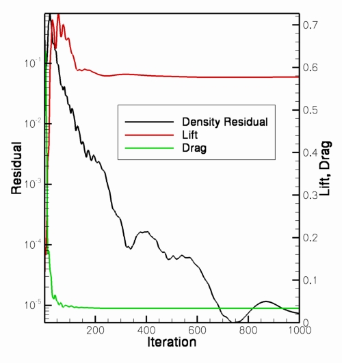
The resulting convergence history is represented in the following plot.
You may also view the resulting f6wbnc.merged_tec_boundary.dat file
with Tecplot.
Zooming in on the symmetry plane,
you will see that the triangular faces have become quad faces,
indicating that the boundary layer grid now consists of prismatic elements.
NASA Official: David P. Lockard
Contact: FUN3D-support@lists.nasa.gov
Page Last Modified: 2026-02-12 17:11:03 -0500
NASA Privacy Statement
Accessibility
This material is declared a work of the U.S. Government and is not subject to copyright protection in the United States.


