Intent: Demonstrate setup and execution of moving overset grids (FUN3D Version 11.0 and higher)

This tutorial will describe how to set up and run a case with moving geometry utilizing overset meshes.

Note: the input data provided in the download files is for FUN3D Version 13.3 and higher and may not work with earlier versions

All the grid and input files may be downloaded below. Note that the grids for this case are very coarse and are intended for demonstration, rather than accurate aerodynamic analysis. The geometry consists of a wing and a store, and is one of the geometries included in SUGGAR++ training materials.

The user should be familiar with running the baseline flow solver, and preferably with running moving geometry cases that don’t require overset grids (See FUN3D Manual: Chapter 7 Grid Motion).

The process is composed of a few basic steps. The download file has a directory structure roughly aligned with these steps. This directory structure is convenient for demonstrating the process, but is not required. First, a composite mesh with the configuration in the initial position is generated from component meshes (in this case wing and store) by running SUGGAR++. The domain connectivity information (dci) for the geometry in the initial position is also computed by SUGGAR++. Next, an initial, steady-state, static geometry computation is performed. The final stage of the tutorial consists of a time-dependent, moving grid computation in which the store motion is specified as a constant downward velocity. The included README files provide step-by-step directions similar to those given on this web page.

Compilation and linking

To use overset grids, you must obtain, compile and link the third-party libraries SUGGAR++ and DiRTlib. See Third-Party Libraries – SUGGAR and Third-Party Libraries – DiRTlib for details.

Files

Download (9.6Mb) and gunzip/untar the files:

Wing_Store/
  README
  Component_Grids/
    store.cogsg
    store.mapbc
    wing.cogsg
    wing.mapbc
    wing.bc
    store.bc
  T=0_Domain_Connectivity/
    Input.xml_0
    README
  Steady_State/
    README
    RUN_IT
    fun3d.nml
  Dynamic_Specified/
    moving_body.input
    README
    RUN_IT
    fun3d.nml

Create the composite mesh and initial domain connectivity information

In this step the component grids, located in the Component_Grids directory, are combined into a single composite VGRID set using SUGGAR++, and at the same time the domain connectivity information is computed for the configuration in the initial t=0 position. Below it is assumed that your suggar++ executable is called suggar++; your executable may be named differently, depending on your compilation platform and compilation options. It is also assumed for illustration purposes that your SUGGAR++ executable is located in a directory /Your/Path/To/Suggar++ The input for SUGGAR++ is provided in the Input.xml_0 file located in the T=0_Domain_Connectivity directory.

  cd Wing_Store/T=0_Domain_Connectivity
  ln -s ../Component_Grids/* .
  ln -s /Your/Path/To/Suggar++/suggar++ .
  (./suggar++ Input.xml_0 > suggar_output) >& suggar_error &

At this point you should have the domain connectivity file wingstore.dci, along with a VGRID file set (wingstore.cogsg, wingstore.mapbc, wingstore.bc) for the composite mesh. You may want to check to see if any orphan points resulted:

  grep "orphans because" suggar_error

You may want to use the GVIZ utility code for SUGGAR++, available from Ralph Noack to view the composite mesh. GVIZ allows visualization of the composite mesh, hole points and fringe points, and can aid in debugging hole-cutting issues. However, it is beyond the scope of this FUN3D tutorial to describe the use of GVIZ.

Steady-state solution

Next, we obtain a steady-state solution for the configuration in the t=0 position. This steady-state solution will be used as the initial solution for the dynamic simulation. A sample run script, RUN_IT, is provided, though it may need modification for your particular system. The run script and fun3d.nml file are such that running FUN3D will generate solution-visualization (TECPLOT) output from within the flow solver. Below, it is assumed that your FUN3D executable (nodet_mpi) is located in /Your/Path/To/Fun3d

  cd ../Steady_State
  ln -s ../T=0_Domain_Connectivity/wingstore.cogsg .
  ln -s ../T=0_Domain_Connectivity/wingstore.mapbc .
  ln -s ../T=0_Domain_Connectivity/wingstore.bc .
  ln -s ../T=0_Domain_Connectivity/wingstore.dci .
  ln -s /Your/Path/To/Fun3d/nodet_mpi .
  ./RUN_IT

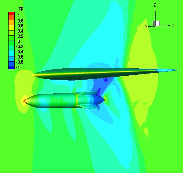
The boundary_animation_freq = -1 and sampling_freq = -1 in fun3d.nml generate TECPLOT output at the end of the flow solver execution. See FUN3D Manual: Appendix B FUN3D Input Files for more information. Here we have used sampling_freq to extract Cp data on a y=0 plane through the flow domain. The boundary_animation_freq is used to extract Cp data on the solid surfaces (wing and store surfaces). Because this is an overset mesh, the default output will contain iblank data. If you have configured FUN3D to link against TECPLOT’s tecio libraries (See FUN3D Manual: Appendix A Installation), then these visualization files will be binary, and will have a .plt or .szplt extension; otherwise, they will be ASCII files and have a .dat extension. The following image was generated from the wingstore_tec_boundary.plt ( .szplt, or .dat) and wingstore_tec_sampling_geom1.plt ( .szplt, or .dat) files. Value blanking on variable iblank was used, with blanking for iblank=0.

Dynamic, moving-grid solution

The steady-state solution obtained above may be used as a starting point for the moving-mesh simulation. Not all moving-mesh simulations need be or in fact can be started from a steady state, although in this case the steady-state initial condition is reasonable. Note that for dynamic overset meshes, not only must the composite mesh be visible to the flow solver, the meshes of all component meshes (static and dynamic) must be visible as well.

  cd ../Dynamic_Specified
  cp ../Steady_State/wingstore.flow .  (note: copy, do not link)
  ln -s ../Component_Grids/* .         (dynamic overset grids need the component grids too)
  ln -s ../T=0_Domain_Connectivity/wingstore.cogsg .
  ln -s ../T=0_Domain_Connectivity/wingstore.mapbc .
  ln -s ../T=0_Domain_Connectivity/wingstore.bc .
  ln -s ../T=0_Domain_Connectivity/wingstore.dci .  (always need the initial dci data)
  ln -s ../T=0_Domain_Connectivity/Input.xml_0 .
  ln -s /Your/Path/To/Fun3d/nodet_mpi .

The motion simulation here is one in which the velocity of the store is specified to be constant, in a downward direction. The moving_body.input file provided in the download tar file is reproduced below:

&body_definitions
  n_moving_bodies = 1,        ! number of bodies in motion
  body_name(1) = 'store',     ! name must be in quotes
  n_defining_bndry(1) = 1,    ! number of boundaries that define this body
  defining_bndry(1,1) = 4,    ! index 1: boundary number index 2: body number
  mesh_movement(1) = 'rigid', ! 'rigid' or 'deform'
  motion_driver(1) = 'forced' ! motion is specified below
/

&forced_motion
  translate(1) = 1,               ! translation type: 1=constant rate 2=sinusoidal
  translation_rate(1) = -0.2,     ! translation velocity (mach)
/

&composite_overset_mesh
  input_xml_file = 'Input.xml_0'
/

See FUN3D Manual: Appendix B FUN3D Input Files for descriptions of all input parameters above. However, a few comments are warranted here. For both the steady-state and time-dependent cases, the ‘patch_lumping = “family”’ option was set in the &raw_grid namelist in the fun3d.nml file. Thus, to the flow solver, the store appears as a single boundary, boundary number 2. It is this lumped boundary numbering that must be used in the &body_definitions namelist above. Because the compressible flow equations in FUN3D are normalized with speed of sound, the specification of the body velocity of -0.2 is equivalent to Mach 0.2 (downward); the freestream Mach number in this case is 0.95.

The input_xml_file is set to be the same Input.xml_0 file that was used with SUGGAR++ to compute the initial (static) DCI data. Note that in this case, in anticipation of running the dynamic simulation, a <dynamic/> element was already placed in the <body name="store"> element at set up time. The “self terminated” <dynamic/> element has no impact on the static grid solution, but does set some additional data that is needed by FUN3D to define which volume grid points are associated with a particular moving body.

The included RUN_IT script for the moving mesh run is reproduced below.

#!/bin/sh
(mpirun -np 9 -nolocal  -machinefile machinefile ./nodet_mpi --temporal_err_control 0.1 --dci_on_the_fly --moving_grid  --overset > screen_output) >& error_output &
exit

Several important points need to be made here. First, note that the command line option --dci_on_the_fly is used trigger a computation of new domain connectivity information at each new time step. This is necessitated by the use of --overset in conjunction with --moving_grid, together with the fact that dci files do not exist a priori for the store mesh at each new position. If the dci files for each time step did already exist, then --dci_on_the_fly would not be needed and they would simply be read in each time step. When --dci_on_the_fly is utilized, the flow solver will write out dci files for each time step; these can be reused for repeat runs, without having to do the (relatively expensive) calculation of the dci data each step. This is most useful in periodic motions, where the flow solver is first run for one period of motion with --dci_on_the_fly. Subsequent restarts omit --dci_on_the_fly and instead use --dci_period N where N is the number of time steps in the period. Note that this example is NOT periodic, so any restarts beyond the 50 time steps in the fun3d.nml file need to be run with --dci_on_the_fly.

Note also that although this example utilizes 8 processors to solve the flow equations, the number of processors used in the mpirun command is 9. When --dci_on_the_fly is used, ONE extra processor is devoted to the task of computing the overset connectivity data. Future versions of the FUN3D and SUGGAR++ are expected to support multiple processors for the dci computation. A very important consequence of the single processor computation of the dci data is that that processor must have sufficient memory to hold the entire mesh on that processor. The SUGGAR++ processor is the first processor in the machinefile list. If the dci files already exist, so that --dci_on_the_fly is not used, the number of processors should be set back to equal the desired number of flow solver processors.

The namelist variable sampling_freq = 5 and boundary_animation_freq = 5 are used to dump out tecplot files much like was done for the steady-state case, except that now the files are generated every 5 time steps. File names contain “_timestepN” to denote which timestep they correspond to. TECPLOT360-2009 was used to generate the animation files below. All .plt ( .szplt, or .dat) files were read with the multiple files option, and in the “Unsteady Flow Options” panel (under the “Analyze” panel) was used to parse the zones by time. Then animation was created using the “Step by Time” option in the “Animation” panel. The first animation shows Cp, analogous to the still image created from the steady-state solution. The second animation shows the dynamic hole cutting as the mesh is moved. To make this animation the mesh was colored by the contour variable imesh. Since there are only two meshes in the composite mesh, all points are either blue (wing) or red (store). Since the mesh in this example is so coarse, the hole cuts tend to be more ragged than with finer meshes, and likewise the contours not as smooth as with finer meshes..

The command-line option—temporal_err_control 0.1 is used to terminate subiterations when the estimate of the temporal error in a time step drops 1 order of magnitude lower than the residual. It is beyond the scope of this tutorial to discuss the theory and potential benefits of this option, but is included here because it is our standard practice for time-accurate simulations. More info can be found in the Training Session materials.