Intent: Demonstrate setup and execution of L/D maximization for steady flow case

This tutorial will describe how to set up and run a shape optimization to maximize the lift-to-drag ratio for steady inviscid flow over a wing at Mach 0.8, alpha=2 degrees. The same procedure applies for viscous/turbulent flow; the user just needs to change the solver inputs accordingly (and the grid/parameterization obviously). Inviscid flow is simply used here for efficiency purposes.

Note: the input data provided in the download files is for FUN3D Version 12.7 and higher and will not work with earlier versions

All of the grid and input files may be downloaded below. Note that the grids for this case are very coarse and are intended for demonstration, rather than accurate aerodynamic analysis. The geometry consists of a single inviscid ONERA M6 wing.

The user should be familiar with running the baseline flow solver.

The process is composed of three basic steps. First, the optimization driver is used to perform an analysis consisting of an evaluation of the surface parameterization, a movement of the volume grid to correspond to that new surface grid, and finally, a flow solution. The next operation demonstrated is using the optimization driver to perform a sensitivity analysis. In this case, the driver will perform an analysis as just described, followed by a flowfield adjoint solution and a mesh adjoint solution to obtain the sensitivity vector. The final portion of the demonstration will use the optimization driver to perform an actual design optimization, maximizing L/D for the baseline wing.

Compilation and linking

To perform design optimization, you must obtain at least one of the third-party optimization libraries covered in the third-party library section of the website (PORT, NPSOL, and/or KSOPT). Your FUN3D installation must be configured and built to use these libraries. If you attempt to run an optimization without building against the library you’re trying to use, the design driver will abort and tell you so. This demo is set up to run using PORT, although KSOPT or NPSOL could be used instead. Since this demo relies on MASSOUD parameterizations, you must also have a MASSOUD executable present in your path.

Files

Download (253 KB).

Set up the baseline directory tree and associated files

The first thing you’ll need to do is create a directory where you wish to run the design case, and go down into it.

mkdir Demo1
cd Demo1

The next step is to use the design driver to construct the directory tree that FUN3D will be expecting to see when it runs the design. Do this by running the driver in your current directory. Note the path in the command is the path to your FUN3D build directory, and the command line argument shown is to generate the directory structure for a single-point design. Enter the required inputs exactly as requested (watch for the single quotes and trailing slashes):

/path/to/your/built/FUN3D/Design/opt_driver --setup_design 1

It is also a good idea to keep the screen output handy, as it is a nice checklist for all of the files you have to have in place prior to starting a design.

Now if you look in your current directory, you will see that the design driver created a tree with several directories. The only ones we will worry about are the description.1 directory (where the baseline case files are stored and never modified during the run) and the ammo directory, where the main optimization is performed from.

First go into the description.1 directory and move the supplied tarfile into here, then untar it:

cd description.1
cp /path/to/tarfile/design_demo1.tar.gz .
gunzip design_demo1.tar.gz
tar xvf design_demo1.tar

You should see the following files extracted into your current (description.1) directory:

command_line.options
design.1
design.gp.1
design.usd.1
fun3d.nml
inviscid.mapbc
inviscid.fgrid
massoud.1
rubber.data

Feel free to look at each file if you want (please do so, in order to get used to what’s in them). Also, look at the command line options for mpirun in the command_line.options file. If those are not what you typically use, then you will need to modify them appropriately. If you are running in a queue environment that automatically handles the number of processors and which machines you will be running on, simply set the number of command line options for mpirun to “0” and delete the options shown in the supplied file.

Next head over to the ammo directory. There you will find the design.nml file which controls the optimization settings. Set your path to the base directory appropriately, and if your MPI implementation is executed using a command other than ‘mpirun’ (such as ‘mpiexec’), then include it as needed. A complete description of the namelist can be found in FUN3D Manual: Chapter 9 Design Optimization.

&design
  base_directory = '/path/to/design/case'
  adjoint_nproc  = 8
/

Perform a baseline analysis using the design driver

Go into the ammo directory and edit the design.nml file. By default, “what_to_do” in the namelist is set to 1, which corresponds to a single analysis at the baseline design variables.

Now enter the following command (if you are running in a queue environment, this is the command that should be placed in your job script):

./opt_driver --sleep_delay 5 > screen.output &

This will fire up the design driver (in the background because of the ampersand at the end of the command) and start to perform a baseline analysis at the initial design point given by the data in the rubber.data file. You can monitor the progress by watching the screen.output file:

tail -f screen.output

Simply hit control-C when you want to exit the tail command.

The first major process you will see go by is party being run to partition the supplied grid.

The next major process you will see is the execution of MASSOUD to evaluate the parameterization at the baseline design point. This is used to define the location of the surface grid.

The next major process (the first MPI process) is the design driver firing off an MPI job to perform a flow solution. The first thing to occur will be a procedure to move the volume grid to conform to the surface grid that MASSOUD just evaluated. One thing to watch for during this step is the initial residual of the linear elasticity solution. It should be very small:

.
.
.
 Iter      Natural Err Est         Error Estimate      Restarts
    0   0.654552664443239E-16   0.000000000000000E+00         0
.
.
.

This indicates that the surface in the baseline volume grid did not need to be moved very much to conform to the baseline design variables. When you do the actual design optimization, you will see this value become some large number, indicating the current surface grid in the volume mesh does not line up with the MASSOUD-generated surface, and therefore the entire mesh will be relaxed into its new position using elasticity relations.

The next major process you will see go by is the actual flow solution. At the end of its execution, you should see the current value of the cost function:

Current value of function            1   176.932025746269

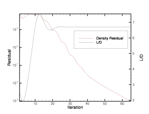
This is the value of the cost function specified in rubber.data at the baseline design variables. If you look at ../model.1/rubber.data, you should now see this value in the cost function field. The usual FUN3D flow solver output files are available in the ../model.1/Flow/ directory. Note that they are also backed up with baseline prefixes, since they will be overwritten at every design cycle during the optimization. If you plot the convergence of the baseline solve we just did using the baseline_hist.dat file, you should get a density residual and L/D convergence that looks something like the following. Note the baseline L/D of about 6.7.

That concludes the baseline analysis procedure. For this very coarse grid (2800 nodes) on 8 processors, this whole process should have taken roughly 30 seconds to complete, depending on your hardware, file system, the sleep_delay you specified, etc.

Perform a baseline sensitivity analysis using the design driver

In this step, we will use the design driver to perform a sensitivity analysis. Edit the design.nml file in the ammo directory, and set “what_to_do” input to 2, which corresponds to a single sensitivity analysis at the baseline design variables.

&design
  base_directory = '/path/to/design/case'
  what_to_do = 2
  adjoint_nproc  = 8
/

As before, now enter the following command:

./opt_driver --sleep_delay 5 > screen.output &

This will fire up the design driver and start to perform a baseline sensitivity analysis at the initial design point given by the data in the rubber.data file. You can monitor the progress by watching the screen.output file.

First, you will see the entire analysis procedure go by as described above.

However, it will now be followed by a couple of additional steps. The first additional step will be another execution of MASSOUD, this time to evaluate the sensitivities of the surface grid location with respect to the design variables. Next you will see an execution of the adjoint solver (dual_mpi) which is solving the adjoint equations for the flowfield, followed by the solution of the mesh adjoint equations. Once the mesh adjoint is solved, the sensitivity analysis procedure is complete. This whole thing should have taken a minute or two, again depending on your hardware and sleep_delay, etc.

Now head over to the ../model.1/Adjoint directory and run Tecplot on the inviscid_hist.dat file. This file contains the convergence history for the flowfield adjoint solution. If you plot the first residual in the file (adjoint equation for continuity), you should see something like the following.

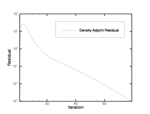
Note the asymptotic convergence is very similar to that of the flow solution. These plots can be used to help set the kickout levels for the flow and adjoint solvers. In general, the kickout levels will be different, since the flow residual scales with the local cell size and the adjoint residual scales with the cost function definition. Also, you typically don’t have to converge the adjoint residuals more than a couple orders of magnitude to get reasonable sensitivities for guiding the optimization.

At this point, all of the sensitivities of the cost function have been populated in the model.1/rubber.data file. Feel free to have a look.

We are now ready to attempt an actual design optimization.

Perform a design optimization using the design driver

Now we will do an actual design optimization. Edit the file design.nml in the ammo directory and change “what_to_do” to “3”. This value will run an actual design.

As before, enter the following command:

./opt_driver --sleep_delay 5 > screen.output &

This will fire up the design driver, and now you will see many analyses and sensitivity analyses going by. You can monitor the progress by watching for the output file(s) specific to the optimizer you are using (see the section on Design), or you can also grep for the current value of the objective function in the screen output:

grep "Current value of function" screen.output

 Current value of function            1   176.932025746269     
 Current value of function            1   136.711111797169     
 Current value of function            1   108.513595498267     
 Current value of function            1   95.8614809311637     
 Current value of function            1   98.9927729907803     
 Current value of function            1   89.8405418971656     
 Current value of function            1   89.8240044903340     
 Current value of function            1   86.9747686981565     
 Current value of function            1   87.2067446771041     
 Current value of function            1   86.4105867018969     
 Current value of function            1   86.0309501312225     
 Current value of function            1   86.4607777183516     
 Current value of function            1   85.6837415868006     
 Current value of function            1   85.7802464741922     
 Current value of function            1   85.3591266402511     
 Current value of function            1   85.3450374750299     
 Current value of function            1   85.3450375806537

Note that in this grep, you will see the cost occasionally go up – these are points in the design space where the optimizer is trying various combinations of the design variables. But in general, the values should be coming down. You can also monitor the cost function field in ../model.1/rubber.data .

When the run finishes (about 5-10 minutes or so, give or take), your final cost function should be roughly 85.35. Since all flow solves were restarted from the previous solution, you can plot up the values in the file ../model.1/Flow/inviscid_hist.dat to reveal the history of the design. You should see something like this for the L/D ratio:

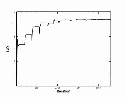
From the plot, you can see that L/D went from the baseline value of 6.7 to roughly 10.76 during the course of the design. The final values of the design variables are given in the ../model.1/rubber.data file.

After the design is complete, you can also animate a history of the surface geometry. Go into the ../model.1/Rubberize/surface_history directory. There you will find a Tecplot file for every body at every step of the optimization. Alternatively, in the Flow directory, you will find a file called movie.tec . This file is a concatenated history of the solutions on the surface throughout the course of the design. This animation of the grid colored by density was created using this file:

From here, you can slice geometries to look at and animate, etc. If you get fancy with the slicing output options in the flow solver, you can do stuff like that, too.

Basically that’s the main steps for doing adjoint-based design optimization with FUN3D…have some patience, and get in touch if you have problems. Good luck!

Intent: Demonstrate setup and execution of multipoint L/D maximization for steady flow case

This tutorial will describe how to set up and run a shape optimization to maximize the lift-to-drag ratio at two separate Mach numbers (0.6 and 0.8) for steady inviscid flow over a wing. The same procedure applies for viscous/turbulent flow; the user just needs to change the solver inputs accordingly (and the grid/parameterization obviously). Inviscid flow is simply used here for efficiency purposes.

The instructions shown here assume the user has gone through the prior design tutorials and understands the basics of how they work.

All of the grid and input files may be downloaded below. Note that the grids for this case are very coarse and are intended for demonstration, rather than accurate aerodynamic analysis. The geometry consists of a single inviscid ONERA M6 wing.

Compilation and linking

This demo is set up to run using PORT. Since this demo relies on MASSOUD parameterizations, you must also have a MASSOUD executable present in your path.

Files

Download (253 KB).

Download (253 KB).

Set up the baseline directory tree and associated files

The first thing you’ll need to do is create a directory where you wish to run the design case, and go down into it.

mkdir Demo2
cd Demo2

The next step is to use the design driver to construct the directory tree that FUN3D will be expecting to see when it runs the design. Do this by running the driver in your current directory. Note the path in the command is the path to your FUN3D build directory, and the command line argument shown is to generate the directory structure for a 2-point design. Enter the required inputs exactly as requested (watch for the single quotes and trailing slashes):

/path/to/your/built/FUN3D/Design/opt_driver --setup_design 2

If you look in your current directory, you will see that the design driver created a tree with several directories. The only ones we will worry about are the description.i directory (where the baseline case files are stored and never modified during the run) and the ammo directory, where the main optimization is performed from.

First go into the description.1 directory and move the supplied tarfile for design point #1 into here, then untar it.

cd description.1
cp /path/to/tarfile/design_demo2_point1.tar.gz .
gunzip design_demo2_point1.tar.gz
tar xvf design_demo2_point1.tar

Now do the same thing for the tar file for design point #2, placing the files into the description.2 directory.

Next head over to the ammo directory. There you will find namelist file design.nml which controls the optimization settings. Edit the file and make it look like the following. Set your path to the base directory appropriately, and if your MPI implementation is executed using a command other than ‘mpiexec’, then include it as needed. The description of the namelist can be found in FUN3D Manual: Chapter 9 Design Optimization.

&design
  base_directory = '/path/to/design/case'
  adjoint_nproc  = 8
  n_design_pts = 2
  what_to_do = 3
  tau_subproblem = 1.0e-5
/

This input deck is going to use PORT to minimize the heuristic multi-point objective function defined to be the sum of the objective function specified in rubber.data in each of the 2 description.i directories. The points are equally weighted.

Perform a multi-point design optimization using the design driver

As before, enter the following command:

./opt_driver --sleep_delay 5 > screen.output &

This will fire up the design driver, and now you will see many analyses and sensitivity analyses going by, some for each design point. You can monitor the progress by watching the ../model.2/port.output file.

When the run finishes (about 20 minutes or so, give or take), your cost function shown in the PORT file should have gone down from roughly 373 to 164. Plotting up the ../model.1/Flow/inviscid_hist.dat and ../model.2/Flow/inviscid_hist.dat files reveals the following history for the L/D ratio at each Mach number:

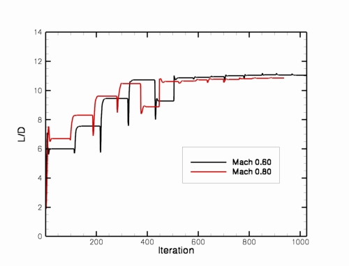
For the Mach 0.60 design point, you can see that L/D went from the baseline value of 6.0 to roughly 11.1 during the course of the design. Similarly, L/D for the Mach 0.80 design point went from 6.7 to 10.9.

Intent: Demonstrate setup and execution of lift-constrained drag minimization for steady flow case

This tutorial will describe how to set up and run a shape optimization to minimize drag subject to a lift constraint for turbulent flow.

The instructions shown here assume the user has gone through the prior design tutorials and understands the basics of how they work. The example shown here is considerably larger (1.8 million grid points) and is demonstrated on 256 processors.

All of the grid and input files may be downloaded below. The grid was originally developed for the 3rd AIAA Drag Prediction Workshop. The geometry is the “Wing 1” configuration, operating at a 0.50 lift coefficient.

Compilation and linking

This demo is set up to run using NPSOL. Since this demo relies on MASSOUD parameterizations, you must also have a MASSOUD executable present in your path.

Files

Download (124 MB).

Download (7.5 MB).

Set up the baseline directory tree and associated files

The first thing you’ll need to do is create a directory where you wish to run the design case, and go down into it.

mkdir Demo3
cd Demo3

The next step is to use the design driver to construct the directory tree that FUN3D will be expecting to see when it runs the design. Do this by running the driver in your current directory. Note the path in the command is the path to your FUN3D build directory, and the command line argument shown is to generate the directory structure for a single-point design. Enter the required inputs exactly as requested (watch for the single quotes and trailing slashes):

/path/to/your/built/FUN3D/Design/opt_driver --setup_design 1

If you look in your current directory, you will see that the design driver created a tree with several directories. The only ones we will worry about are the description.i directory (where the baseline case files are stored and never modified during the run) and the ammo directory, where the main optimization is performed from.

First go into the description.1 directory and move the first supplied tarfile (the big one containing the grid from the DPW-3 website ) into here, then untar it.

cd description.1
cp /path/to/tarfile/Grid_dpww1_0.6_dist.tar.gz .
gunzip Grid_dpww1_0.6_dist.tar.gz
tar xvf Grid_dpww1_0.6_dist.tar

Now move the second supplied tarfile into here, then untar it also.

cp /path/to/tarfile/design_demo3.tar.gz .
gunzip design_demo3.tar.gz
tar xvf design_demo3.tar

Note that there is a replacement .mapbc file in the second tar file to override the one supplied on the DPW site. The only difference is the boundary condition on the symmetry plane, which for our purposes here, should be set to 3080 (sliding tangency).

If you examine the supplied rubber.data file, you will see two functions defined. One is the explicit lift constraint with a lower bound of 0.50, and the other is the objective function, based on the drag coefficient. Note that a weighting parameter has been used on both to scale the typical values of the functions to order-1 quantities. I’ve found that this often helps NPSOL move the design along better. Constrained optimization is still very much an art though, and I would encourage you to play with settings and see what works on your cases.

You will see that we are using 107 design variables for this case – angle of attack plus a bunch of camber and thickness variables describing the wing shape. The thickness bounds are set such that no thinning of the wing is allowed.

Next head over to the ammo directory. There you will find a template for the ammo.input file which controls the optimization settings. Edit the file and make it look like the following. Set your path to the base directory appropriately, and if your MPI implementation is executed using a command other than ‘mpirun’ (such as ‘mpiexec’), then include it as needed. Note that in the supplied example I have not included any command line options for the mpirun command. I ran this job in a queuing environment which handles all of the MPI runtime options for me.

Optimization package
5
Base directory from which to run optimization
'/misc/work13/nielsen/12.2Tutorials/DemoIV.3/Demo3'
Number of design points
1
Weights for each design point
1.0
Operation to perform
3
Restart the optimization
0
Diagnostics flag
0
Maximum number of lo-fi functions per subproblem
30
Maximum number of lo-fi subproblem iterations
20
Relative convergence criterion for subproblem
1.e-5
Absolute feasibility tolerance for constraint violation
0.01
Number of bodies with spatial transforms
1
List of bodies with spatial transforms
1
Body grouping desired (0=no, 1=yes)
0
Executable for running MPI programs
'mpirun'
Number of processors from which to run adjoint solver
256
DOT method (see DOT documentation)
0

Perform a lift-constrained drag minimization using the design driver

As before, enter the following command:

./opt_driver --sleep_delay 30 > screen.output &

This will fire up the design driver, and the design process will start up. You can monitor the progress by watching the screen.output file.

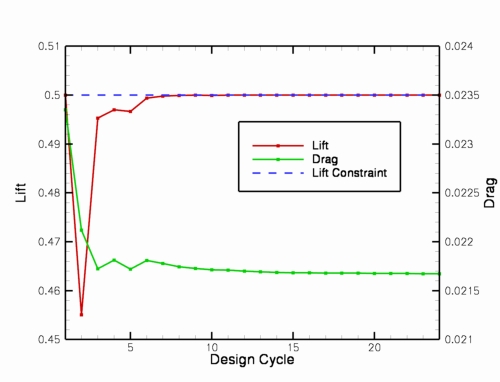
When the run finishes (about 10 hours or so, depending on your hardware – the optimizer will call the flow and adjoint solvers about 20 times each), you should get a npsol.printfile and a npsol.summaryfile in your top-level directory. You should see that the objective function has decreased from 5.45 to roughly 4.70, while the constraint is met with a lift coefficient of 0.50. The drag has been reduced roughly 16 counts, from 0.0233 to 0.0217. Plotting up the ../model.1/Flow/forces.tec file (simple file that contains lift, drag, L/D history during the design) reveals the following history for the lift and drag coefficients.

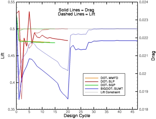
We also demonstrate the use of the DOT and BIGDOT packages for performing the same case. These packages can be used in the exact same manner in which NPSOL was used above, with the exception of how the lift constraint is specified. Since DOT/BIGDOT require constraints to be of the form g.le.0, we must alter the functional form specified in rubber.data as follows:

.
.
.
Components of function   2: boundary id (0=all)/name/value/weight/target/power
    0 cl            0.000000000000000   -10.  0.50000 1.000
.
.
.

Note that we have retained the weight value of 10 to keep the nominal function value on the order of 1. Also, when using DOT/BIGDOT, the value of the constraint is rolled into the function definition, so the lower and upper constraint bounds specification a few lines above this in rubber.data is irrelevant for such cases. The results obtained by trying each of the methods available in DOT/BIGDOT are shown in the plot below. Note that in general, results will be problem-dependent, so one should not infer general trends from this one case.

Intent: Demonstrate setup and execution of L/D maximization for unsteady pitching wing case

This tutorial will describe how to set up and run a shape optimization to maximize the lift-to-drag ratio over a pitching cycle for unsteady inviscid flow over a wing at Mach 0.3, with a 5-deg pitching amplitude about a 0-deg mean. The same procedure applies for viscous/turbulent flow; the user just needs to change the solver inputs accordingly (and the grid/parameterization obviously). Inviscid flow is simply used here for efficiency purposes.

Note: the input data provided in the download files is for FUN3D Version 12.7 and higher and will not work with earlier versions

All of the grid and input files may be downloaded below. Note that the grids for this case are very coarse and are intended for demonstration, rather than accurate aerodynamic analysis. The geometry consists of a single inviscid ONERA M6 wing.

The user should be familiar with running the baseline unsteady flow solver for moving mesh cases and all of the steady design optimization capabilities. Although this tutorial case is quite cheap, please do not attempt unsteady design optimization without plenty of computing resources available. The algorithms are very efficient, but the cost will still be the equivalent of many unsteady solutions for your problem.

The instructions included here simply lead the user through the optimization procedure. You may still use the framework to perform just an analysis or a sensitivity analysis as in the steady case (and it is highly recommended that you do).

Compilation and linking

This demo is set up to run using PORT, although KSOPT or NPSOL could be used instead. Since this demo relies on MASSOUD parameterizations, you must also have a MASSOUD executable present in your path.

Files

Download (255 KB).

Set up the baseline directory tree and associated files

The first thing you’ll need to do is create a directory where you wish to run the design case, and go down into it.

mkdir Demo4
cd Demo4

The next step is to use the design driver to construct the directory tree that FUN3D will be expecting to see when it runs the design. Do this by running the driver in your current directory. Note the path in the command is the path to your FUN3D build directory, and the command line argument shown is to generate the directory structure for a single-point design. Enter the required inputs exactly as requested (watch for the single quotes and trailing slashes):

/path/to/your/built/FUN3D/Design/opt_driver --setup_design 1

It is also a good idea to keep the screen output handy, as it is a nice checklist for all of the files you have to have in place prior to starting a design.

Now if you look in your current directory, you will see that the design driver created a tree with several directories. The only ones we will worry about are the description.1 directory (where the baseline case files are stored and never modified during the run) and the ammo directory, where the main optimization is performed from.

First go into the description.1 directory and move the supplied tarfile into here, then untar it:

cd description.1
cp /path/to/tarfile/design_demo4.tar.gz .
gunzip design_demo4.tar.gz
tar xvf design_demo4.tar

You should see the following files extracted into your current (description.1) directory:

command_line.options
design.1
design.gp.1
design.usd.1
fun3d.nml
inviscid.fgrid
inviscid.mapbc
massoud.1
moving_body.input
rubber.data

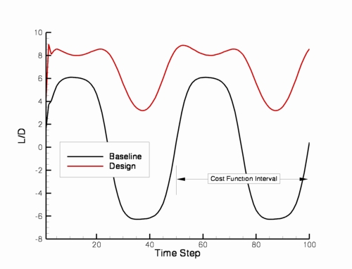
Feel free to look at each file if you want (please do so, in order to get used to what’s in them). Note the cost function in rubber.data is specified to be the sum of the squared differences between L/D and a target value of 20 over timesteps 51-100 (the second pitch cycle – to allow transients from the first pitching cycle to wash out).

The only files from the tar file that should need modifications are as follows. If needed for your system, you will need to include the appropriate command line options for mpirun in the command_line.options file. Next head over to the ammo directory. There you will find a template for the design.nml file which controls the optimization settings. Edit the file and make it look like the following. Set your path to the base directory appropriately, and if your MPI implementation is executed using a command other than ‘mpiexec’, then include it as needed. A complete description of the namelist can be found in FUN3D Manual: Chapter 9 Design Optimization.

&design
  base_directory = '/path/to/design/case'
  adjoint_nproc  = 8
  what_to_do = 3
  tau_subproblem = 1.0e-4
  max_design_cycles = 20
  max_function_evals = 30
  mpirun_prefix = 'mpirun'
/

Perform a design optimization using the design driver

As before, enter the following command:

./opt_driver --sleep_delay 5 > screen.output &

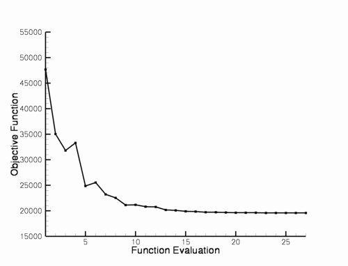
This will fire up the design driver, and you will see many unsteady analyses and sensitivity analyses going by. You can monitor the progress by watching for the output file(s) specific to the optimizer you are using (see the section on Design), or you can also grep for the current value of the objective function in the screen output:

grep "Current value of function" screen.output

 Current value of function            1   47701.1063544135     
 Current value of function            1   35052.4726444651     
 Current value of function            1   31811.4616316012     
 Current value of function            1   33342.7312645150     
 Current value of function            1   24866.3041072219     
 Current value of function            1   25553.1573524893     
 Current value of function            1   23231.8856550912     
 Current value of function            1   22574.2990086534     
 Current value of function            1   21157.8724441327     
 Current value of function            1   21203.7407878034     
 Current value of function            1   20841.2188175691     
 Current value of function            1   20796.6054491425     
 Current value of function            1   20180.0004236392     
 Current value of function            1   20107.2923574798     
 Current value of function            1   19908.8900206760     
 Current value of function            1   19896.6976624663     
 Current value of function            1   19752.0784780769     
 Current value of function            1   19724.5576859762     
 Current value of function            1   19708.5998944041     
 Current value of function            1   19646.0396535845     
 Current value of function            1   19650.5851963433     
 Current value of function            1   19632.9182261230     
 Current value of function            1   19617.6665410400     
 Current value of function            1   19613.4528200157     
 Current value of function            1   19606.1060622060     
 Current value of function            1   19596.7081536189     
 Current value of function            1   19596.7081542119

Note that in this grep, you will see the cost occasionally go up – these are points in the design space where the optimizer is trying various combinations of the design variables. But in general, the values should be coming down. You can also monitor the cost function field in ../model.1/rubber.data .

When the run finishes (about 50 minutes or so on 8 processors, give or take), your final cost function should be roughly 21275. Unlike for steady flows, the flow solver is always started from freestream for unsteady optimizations. Therefore you can plot up the original vs designed values using the files ../model.1/Flow/baseline_hist.dat and ../model.1/Flow/inviscid_hist.dat . You should see something like this for the L/D ratio:

The final values of the design variables are given in the ../model.1/rubber.data file. The final wing has been cambered significantly:

Intent: Demonstrate setup and execution of L/D maximization for steady flow case using Sculptor

This tutorial will describe how to set up and run a shape optimization to maximize L/D for turbulent flow using Sculptor.

The instructions shown here assume the user has gone through the prior design tutorials and understands the basics of how they work. The example shown here is somewhat large (672,000 grid points) and is demonstrated on 128 processors.

All of the grid and input files may be downloaded below. The grid was originally developed for the 4th AIAA Drag Prediction Workshop. Note the mesh is extremely coarse and is not necessarily intended to resolve all of the pertinent flow physics.

Compilation and linking

This demo is set up to run using PORT. Since this demo relies on Sculptor, you must also have Version 3.1 or later of Sculptor installed and functional.

Files

Download (107 MB).

Download (2.9 MB).

Set up the baseline directory tree and associated files

The first thing you’ll need to do is create a directory where you wish to run the design case, and go down into it.

mkdir Demo5
cd Demo5

The next step is to use the design driver to construct the directory tree that FUN3D will be expecting to see when it runs the design. Do this by running the driver in your current directory. Note the path in the command is the path to your FUN3D build directory, and the command line argument shown is to generate the directory structure for a single-point design. Enter the required inputs exactly as requested (watch for the single quotes and trailing slashes):

/path/to/your/built/FUN3D/Design/opt_driver --setup_design 1

If you look in your current directory, you will see that the design driver created a tree with several directories. The only ones we will worry about are the description.i directory (where the baseline case files are stored and never modified during the run) and the ammo directory, where the main optimization is performed from.

First go into the description.1 directory and move the first supplied tarfile (the big one containing the grid from the DPW-4 website ) into here, then untar it.

cd description.1
cp /path/to/tarfile/dpw-wbt0_crs-3.5Mc_5.tgz .
tar xvfzl dpw-wbt0_crs-3.5Mc_5.tgz

Now move the second supplied tarfile into here, then untar it also.

cp /path/to/tarfile/design_demo5.tar.gz .
gunzip design_demo5.tar.gz
tar xvf design_demo5.tar

Note that there is a replacement .mapbc file in the second tar file to override the one supplied on the DPW site. The only difference is the boundary condition on the symmetry plane, which for our purposes here, should be set to 3080 (sliding tangency).

If you examine the supplied rubber.data file, you will see that the cost function is based on the lift-to-drag ratio, with an arbitrarily large target value of 25. The baseline L/D for this case is 8.8. We do not expect the optimization to reach 25, but we will let it do what it can.

You will see that we are using 94 shape design variables for this case, according to the Sculptor files that have been set up ahead of time. For details on how to use Sculptor, the reader is referred to the documentation for that software. Note that Sculptor has been used to parameterize both the wing and the tail surfaces, but they must be contained within the same instance of files, and FUN3D sees all of the design variables as a single concatenated list in rubber.data.

Next head over to the ammo directory. There you will find a template for the ammo.input file which controls the optimization settings. Edit the file and make it look like the following. Set your path to the base directory appropriately, and if your MPI implementation is executed using a command other than ‘mpirun’ (such as ‘mpiexec’), then include it as needed. Note that in the supplied example I have not included any command line options for the mpirun command. I ran this job in a queuing environment which handles all of the MPI runtime options for me.

Optimization package
4
Base directory from which to run optimization
'/misc/work13/nielsen/Demo5'
Number of design points
1
Weights for each design point
1.0
Operation to perform
3
Restart the optimization
0
Diagnostics flag
0
Maximum number of lo-fi functions per subproblem
30
Maximum number of lo-fi subproblem iterations
20
Relative convergence criterion for subproblem
1.e-5
Absolute feasibility tolerance for constraint violation
110.0
Number of bodies with spatial transforms
0
List of bodies with spatial transforms
Body grouping desired (0=no, 1=yes)
0
Executable for running MPI programs
'mpirun'
Number of processors from which to run adjoint solver
128
DOT Method
0

Perform a maximization of L/D ratio using the design driver

As before, enter the following command:

./opt_driver --sleep_delay 30 > screen.output &

This will fire up the design driver, and the design process will start up. You can monitor the progress by watching the screen.output file.

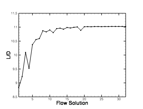
When the run finishes (about 1-2 hours or so, depending on your hardware – the optimizer will call the flow solver about 30 times and the adjoint about 20 times), you should get a port.output file in your top-level model.1 directory. You should see that the objective function has decreased from 261.4 to roughly 195.3. Plotting up the ../model.1/Flow/forces.tec file (simple file that contains lift, drag, L/D history during the design) reveals the following history for the lift-to-drag ratio. L/D has gone from its baseline value of 8.8 to a value of 11.0.